Before 2017, AI had a fundamental problem: neural networks could only read text one word at a time, like following your finger across a page. By the time they reached the end of a long sentence, they'd forgotten the beginning.

This killed performance on everything that mattered - translation, conversation, writing. The best language models were like readers with severe memory problems.

Then Google published Attention Is All You Need. The core insight: what if every word could look at every other word simultaneously?

That simple idea broke the sequential bottleneck and unleashed ChatGPT, GPT-4, and the entire AI revolution we're living through today.

The big idea: parallel processing for language

The Transformer's core breakthrough is relatively simple: instead of processing "The cat sat on a mat" word by word, it looks at all six words simultaneously and lets them figure out their relationships to each other.

"Attention Is All You Need" made one bold claim: you don't need recurrent or convolutional layers at all. Just attention mechanisms.

We propose a new simple network architecture, the Transformer, based solely on attention mechanisms, dispensing with recurrence and convolutions entirely. (Vaswani et al., 2017)

The authors weren't trying to build a better RNN - they were proposing to eliminate sequential processing entirely. Every word gets to "attend" to every other word in parallel, asking: "Which of these other words are relevant to understanding me?"

This parallel processing changed AI in two ways: it delivered speed (no token-by-token bottleneck) and preserved long-range context.

The result? Models that could finally understand language the way humans do - holistically, with full context, all at once.

How the attention mechanism works

To understand how this parallel processing actually works, we need to start with how computers represent words as numbers.

What is an embedding?

Computers can't work with words directly - they only understand numbers. So before we can apply attention, we need to convert words like "cat" and "sat" into numerical representations that capture their meaning.

This is where embeddings come in. An embedding transforms each word into a high-dimensional vector of numbers. Words with similar meanings get similar vectors - "cat" and "dog" will have embeddings that are closer together than "cat" and "airplane."

In short, you can think of an embedding as a vector (a list of numbers) that represents the meaning of a word.

If we have a sentence of, say, 6 words, and each word is represented as a vector of size 512 then our whole sentence becomes a matrix of shape (6, 512).

Query, key and value

For attention to work, each word needs to play three different roles:

• Query: "What am I looking for?" (What information does this word need?)
• Key: "What do I represent?" (What information can this word provide?)
• Value: "What information do I actually contain?" (The actual content to share)

Think of it like a database: the query asks a question, keys indicate what each record contains, and values are the actual data returned.

The Transformer creates these three different "views" of each word by learning to transform the original embedding. Let's work with concrete numbers: if our word embeddings are 512 numbers each, we might transform them into query, key, and value vectors that are each 64 numbers long.

Why these specific numbers? The original "Attention Is All You Need" paper used 512-dimensional embeddings and 64-dimensional query/key/value vectors, so we'll follow their example.

To make this transformation, the Transformer learns three weight matrices:

• One to turn the embedding into a query vector
• One to turn it into a key vector
• One to turn it into a value vector

Here's how the math works: to transform a 512-number embedding into a 64-number query vector, we need a weight matrix of shape (512 × 64). The same logic applies to keys and values:

W_Q: shape (512 × 64)
W_K: shape (512 × 64)
W_V: shape (512 × 64)

Each matrix takes our 512-dimensional word embedding and projects it into a different 64-dimensional space - one for queries, one for keys, one for values.

The same original vector (like for "sat") gets multiplied by each of these three matrices to give three different projections of the same word - the query, key, and value.

A note on shapes: Each word embedding starts as a 1D vector (512,). For matrix multiplication, it's treated as (1, 512) and multiplied by a (512, 64) weight matrix, resulting in (1, 64). Whether we keep or squeeze the extra dimension depends on the framework, but the key idea remains: we’re projecting 512-dimensional embeddings into 64-dimensional Q/K/V spaces.

Let's verify this with actual numbers to see the dimensionality transformation in action:

import numpy as np

# Start with a 512-dimensional word embedding
embedding = np.random.rand(512)
print(f'Word embedding shape: {embedding.shape}')

# Weight matrix to transform into 64-dimensional space
W_Q = np.random.rand(512, 64)
print(f'Weight matrix shape: {W_Q.shape}')

# Transform embedding into query vector
query = embedding @ W_Q
print(f'Query vector shape: {query.shape}')

# Same process creates key and value vectors
W_K = np.random.rand(512, 64)
W_V = np.random.rand(512, 64)
key = embedding @ W_K
value = embedding @ W_V

print(f'Each word gets: Query{query.shape}, Key{key.shape}, Value{value.shape}')

We repeat this for every word in the sentence - each word gets its own query, key and value vector.

Now we can use these to compute how much attention one word should pay to others.

Single attention head walkthrough

Let’s suppose we’re updating the embedding for the word "sat". We already have its query vector:

query_sat = embedding("sat") @ W_Q  → shape (64,)

Now, for each word in the sentence (including "sat" itself), we have a key vector:

key_the  = embedding("the")  @ W_K
key_cat  = embedding("cat")  @ W_K
key_sat  = embedding("sat")  @ W_K
key_on   = embedding("on")   @ W_K
key_a    = embedding("a")  @ W_K
key_mat  = embedding("mat")  @ W_K

To compute how much "sat" should attend to "cat", "mat", etc., we take the dot product of query_sat with each key vector:

score_the  = query_sat • key_the
score_cat  = query_sat • key_cat
score_sat  = query_sat • key_sat
...

The dot product operation is simple: multiply corresponding elements of two vectors, then add them up. For a dot product to work, both vectors must have exactly the same number of elements (same dimensionality).

These are raw attention scores - higher means more relevance.

We then divide them all by $\sqrt{64}$ (square root of key size) to prevent the dot-product scores from blowing up as the key dimension grows. This keeps the softmax outputs from collapsing onto a single word.

scaled_scores = [score_the, score_cat, ...] / √64

What would happen if we didn't divide it $\sqrt{64}$?

Let's see it in code.

import numpy as np

def softmax(x):
  exps = np.exp(x)
  return exps / np.sum(exps)

np.set_printoptions(precision=3, suppress=True)

np.random.seed(0)
q = np.random.randn(64)
k = np.random.randn(6, 64)

scores = k @ q
print("Unscaled:", softmax(scores))
print("Scaled:  ", softmax(scores / np.sqrt(64)))

Without scaling, one weight tends to dominate and the distribution becomes very peaky, so almost every other word is effectively ignored. Dividing by $\sqrt{64}$ keeps more words in play.

Then we pass those scaled scores through a softmax, which turns them into attention weights that sum to 1:

attention_weights = softmax(scaled_scores)

Now we have attention weights that tell us how much "sat" should focus on each word. But we're not done - we need to use these weights to create a new embedding for the word "sat".

This is where the value vectors come in. Each word's value vector gets multiplied by its attention weight, then we sum them all up:

new_embedding_sat = 
  attention_weight_the × value_the +
  attention_weight_cat × value_cat +
  attention_weight_sat × value_sat +
  attention_weight_on × value_on +
  attention_weight_a × value_a +
  attention_weight_mat × value_mat

The result is this attention head's output for "sat" that incorporates information from all relevant words in the sentence, weighted by their importance according to this particular head's learned attention pattern.

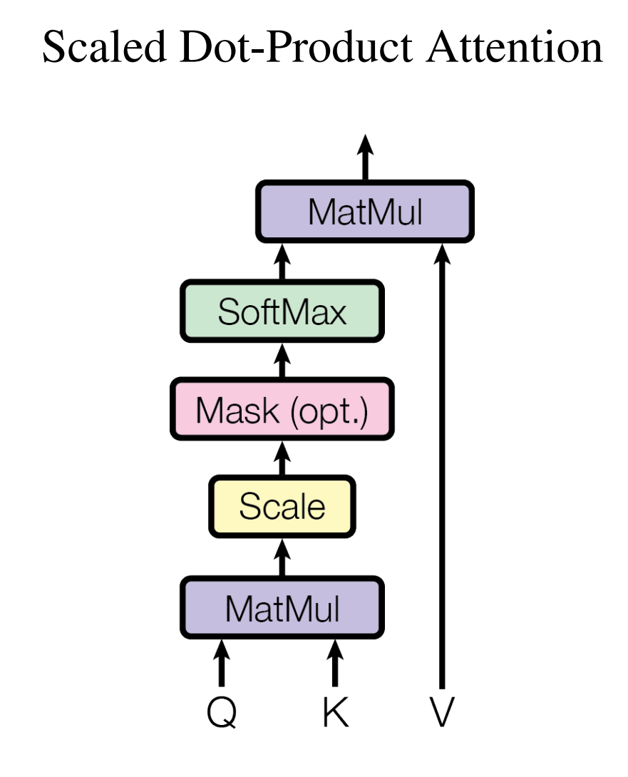
This diagram shows the exact computational flow we just walked through step by step. The MatMul operations represent the dot products, Scale divides by $\sqrt{d_k}$, SoftMax normalizes the attention weights, and the final MatMul with $V$ produces the weighted sum of values.

Multi-head attention

Wait - we have a problem. Our attention head outputs a 64-dimensional vector, but we started with a 512-dimensional embedding. How do we get back to the original size? We could use a different approach with larger Q, K, V matrices, but the Transformer does something more elegant.

Here's the trick: we don’t just have one attention head. We have multiple heads - say, 8.

Every attention head gets its own $W_Q$, $W_K$, and $W_V$.

Each head gives you a 64-dimensional output. So now we have:

head_1: (64,)
head_2: (64,)
...
head_8: (64,)

We concatenate all these outputs, and now we're back to the full embedding size.

But why do we need 8 different heads doing what seems like the same thing?

Each attention head learns to focus on different types of relationships. Think of them as specialists: one head might learn to connect subjects with their verbs (like "cat" → "sat"), while another focuses on objects and their prepositions ("mat" → "on"). A third head might track long-distance dependencies across clauses, and yet another might specialize in detecting negations or modifiers.

This specialization happens naturally during training - we don't explicitly tell each head what to focus on. The model discovers that having multiple "attention perspectives" gives it a richer understanding of language relationships. It's similar to how different parts of your brain process different aspects of what you see: one area focuses on edges, another on colors, another on motion. Multi-head attention gives the Transformer multiple ways to parse the same sentence simultaneously.

Finally, we pass that through one final matrix multiplication:

output = concat_output @ W_O

where $W_O$ is a weight matrix of shape (512, 512).

But why do we need this final transformation? The concatenated output from all heads is just 8 different 64-dimensional vectors stuck together. Each head learned its own specialized patterns, but now we need to combine and integrate all that information.

​$W_O$ learns how to mix and weight the contributions from each attention head. It might decide that head 1's subject-verb connections are more important than head 3's long-distance dependencies for this particular context. Or it might learn to combine insights from multiple heads in sophisticated ways.

Without $W_O$, we'd just have 8 separate attention outputs sitting side by side with no interaction. The output projection lets the model learn how to synthesize all those different attention perspectives into a single, coherent representation.

There is another architectural detail we can take away from this: we need to coordinate the number of attention heads with the size of the QKV vectors. The rule is:

embedding size = number of heads × QKV vector size

So if our embedding is 512, and we want 8 heads, then each head's query, key and value vectors must be 64-dimensional.

Why?

Because after we compute the output from each head (shape 64), we concatenate all of them:

concat_output = [head_1, head_2, ..., head_8] → shape: (512,)

This way, the concatenated result perfectly fits into the expected shape for the next layer.

If we wanted 16 heads, then each head would use QKV of size 32.

The attention formula

Now that we've walked through each step of the attention mechanism, let's see how all of this can be expressed in a single, elegant mathematical formula.

Remember what we computed step by step:

1. Take dot products between the query and all keys
2. Scale by $\sqrt{d_k}$
3. Apply softmax to get attention weights
4. Use those weights to mix the value vectors

All of these operations can be written compactly using matrix notation. Instead of computing attention for one word at a time, we can process the entire sequence simultaneously by organizing our queries, keys, and values into matrices.

Where:

• $Q$ is the query matrix containing query vectors for all words in the sequence
• $K^T$ is the key matrix (transposed) containing all the key vectors
• $d_k = 64$ is the dimension of our key vectors
• $V$ is the value matrix containing all the value vectors
• The result is a matrix where each row is the weighted sum of value vectors for each word

The complete multi-head attention architecture

Now let's see how all these pieces fit together in the actual Transformer architecture:

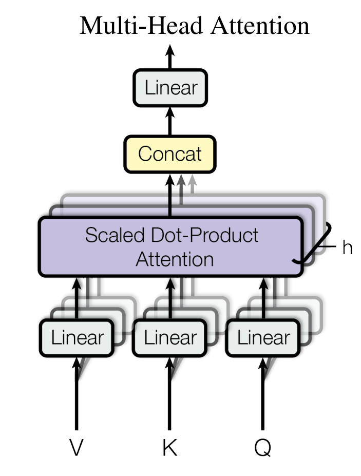
This diagram shows how multi-head attention works, but let's clarify what's happening.

The three arrows labeled $V$, $K$, $Q$ at the bottom all represent the same input - the original word embeddings from our sentence. In this post we’re describing self-attention, where $Q$, $K$, and $V$ are all projections of the same input sequence $X$.

Each gets processed through a different Linear transformation:

• Left Linear: Transforms input embeddings using $W_V$ to create value vectors
• Middle Linear: Transforms input embeddings using $W_K$ to create key vectors
• Right Linear: Transforms input embeddings using $W_Q$ to create query vectors

The diagram shows V, K, Q as separate inputs, but they're actually all the same input embeddings transformed through different Linear layers.

Remember, this entire structure gets replicated for each attention head (8 times in the original paper). Each head learns its own $W_Q$, $W_K$, and $W_V$ matrices, so each head can focus on different types of relationships.

The "h" on the right indicates that this block runs in parallel h times (once per head), then all outputs get concatenated and passed through the final Linear layer ($W_O$).

Wrapping up

We started with neural networks that forgot the beginning of a sentence by the time they reached the end. The Transformer's solution was to let every word look at every other word simultaneously through the attention mechanism.

The core mechanics are queries finding relevant keys, attention weights mixing values, and multiple heads capturing different relationships. It's a relatively simple idea that changed how we build language models.

I hope this walkthrough helped clarify how self-attention actually works under the hood. If you spot any errors or have suggestions for explaining this better, I'd love to hear from you - reach out on X or LinkedIn.

Thanks for reading, and thanks to the researchers who made this breakthrough possible.

Further reading

• Attention Is All You Need (Vaswani et al., 2017) - The foundational paper that introduced the Transformer architecture. Essential reading to see the original motivation and mathematical formulation.
• The Illustrated Transformer by Jay Alammar - Beautifully illustrated walkthrough of the complete Transformer architecture with excellent visual explanations.
• The Annotated Transformer by Harvard NLP - Line-by-line implementation of the Transformer with detailed explanations of each component.
• Flash Attention (Dao et al., 2022) - Modern optimization of attention computation that makes long sequences tractable.
• BertViz - Tool for visualizing attention patterns in BERT and other Transformer models.